Every atom of carbon in your body was once inside a star. The nuclear furnaces of dying red giants fused three helium nuclei into carbon through a reaction so improbable that the physicist Fred Hoyle predicted a previously unknown energy resonance in the carbon-12 nucleus to explain why the element exists in such abundance. That resonance, confirmed experimentally in 1957, is a reminder that carbon's role in the story of life and climate is not merely chemical but cosmological. The universe conspired, through the fine-tuning of nuclear physics, to produce the one element capable of building molecules complex enough to encode information, catalyse reactions, store energy, and circulate through a planet's oceans, atmosphere, rocks, and biosphere in cycles that span seconds to hundreds of millions of years.
The material moves beyond the foundational picture of carbon's reservoirs and fluxes into the deeper architecture that governs how carbon behaves at the molecular level, how scientists measure its movements with precision, and how the global carbon budget constrains civilisation's options. The fast carbon cycle and the slow geological cycle are examined here as coupled components of a single planetary engine whose behaviour under human perturbation depends on chemical kinetics, isotopic signatures, ocean buffering capacity, and the relentless arithmetic of residence times. The carbon budget equation is unpacked here into the physical and biological mechanisms that determine each term, and the consequences of those mechanisms for the remaining carbon space within which climate targets must be achieved.
The tools of this analysis range from the quantum mechanics of molecular vibration that makes carbon dioxide a greenhouse gas to the satellite instruments that now map carbon fluxes across entire continents. Understanding the carbon cycle at this level of detail is not an exercise in academic completeness. It is the prerequisite for evaluating every claim, every policy, and every technology that bears on the question of whether civilisation can bring its carbon emissions into balance with the planet's capacity to absorb them.
The Molecular Architecture of Carbon
Orbital Hybridisation and the Geometry of Bonding
Carbon's extraordinary chemical versatility arises from a property that introductory chemistry often states but rarely explains: its ability to form four covalent bonds simultaneously. The explanation lies in the quantum mechanics of its electron configuration. A ground-state carbon atom has its six electrons arranged as 1s² 2s² 2p², which would suggest two bonds from the two unpaired 2p electrons. In practice, carbon undergoes orbital hybridisation, a process in which the 2s and 2p orbitals mix to form new hybrid orbitals of equivalent energy. In the most common hybridisation, called sp³, one s orbital and three p orbitals combine to produce four identical sp³ hybrid orbitals arranged in a tetrahedron, with bond angles of approximately 109.5 degrees. This is the geometry of methane, of diamond, and of the saturated carbon backbone in fats and sugars.
When carbon forms double bonds, it uses sp² hybridisation: three hybrid orbitals lie in a plane at 120-degree angles, while the remaining unhybridised p orbital extends above and below the plane, forming the second bond of the double bond through lateral overlap. Carbon dioxide is the linear case: each carbon-oxygen bond arises from one sigma bond in the sp framework and one pi bond from a perpendicular p orbital, which is why the molecule is linear rather than bent. In triple bonds, sp hybridisation produces two bonds at 180 degrees with two perpendicular pi bonds, as in carbon monoxide or acetylene. The range of hybridisation states gives carbon access to linear, planar, and three-dimensional geometries simultaneously, and it is this geometric flexibility, as much as the number of bonds, that enables the millions of distinct organic molecules that carbon forms.
The bond energies involved are central to understanding why carbon compounds dominate both biology and energy. A carbon-carbon single bond has a bond energy of approximately 346 kilojoules per mole, strong enough to build stable chains and rings yet weak enough to be broken enzymatically during metabolism. A carbon-oxygen double bond in carbon dioxide has a bond energy of approximately 799 kilojoules per mole, reflecting the stability of the molecule and the energy required to break it during photosynthesis. The carbon-hydrogen bond, at roughly 411 kilojoules per mole, stores chemical energy in a compact form, which is why hydrocarbons release so much heat when oxidised. These numbers are not abstract thermodynamic curiosities. They are the reason fossil fuels are energy-dense, the reason photosynthesis requires sunlight as an energy input, and the reason that reversing combustion to recapture carbon dioxide from the atmosphere is thermodynamically costly.
Carbon's Allotropes and the Spectrum of Solid Forms
The same element that forms the backbone of soft fats and fragile sugars also constitutes the hardest natural material on Earth. Carbon's solid forms, its allotropes, span a range of structures and properties that no other element matches. In diamond, every carbon atom is sp³ hybridised and bonded to four neighbours in a rigid three-dimensional lattice, producing extreme hardness, optical transparency, and electrical insulation. In graphite, carbon atoms are sp² hybridised in flat hexagonal sheets, with weak van der Waals forces between layers allowing them to slide over one another, which is why graphite is soft, opaque, and useful as a lubricant and pencil lead. The delocalised pi electrons in graphite's sheets also make it an electrical conductor along the plane of the layers, a property exploited in electrodes and batteries.
The discovery of fullerenes in 1985 by Harold Kroto, Robert Curl, and Richard Smalley revealed that carbon could form closed cage structures, the most famous being buckminsterfullerene (C₆₀), a truncated icosahedron resembling a football. Graphene, a single layer of graphite isolated experimentally in 2004 by Andre Geim and Konstantin Novoselov, proved to be the strongest material ever measured, with a tensile strength over 100 times that of steel, along with remarkable electrical and thermal conductivity. Carbon nanotubes, essentially rolled sheets of graphene, exhibit properties that depend on the angle of rolling, a geometric detail that determines whether the tube conducts electricity like a metal or behaves as a semiconductor. These discoveries have transformed materials science, but from the perspective of the carbon cycle, the relevant insight is that carbon's bonding flexibility allows it to exist stably in forms ranging from atmospheric gases to minerals locked in rock for hundreds of millions of years, and that the energy barriers between these forms define the timescales over which carbon moves through the planet. The transformation of graphite into diamond requires pressures exceeding 5 gigapascals and temperatures above 1,500 degrees Celsius, conditions found at depths of roughly 150 kilometres in Earth's mantle, which is why natural diamonds are geological rarities brought to the surface by volcanic eruptions. The combustion of coal (predominantly sp²-bonded carbon) into carbon dioxide requires only a match and the oxygen in the air, which is why fossil fuels can be burned so easily and why the rate of geological carbon release through industrial combustion so dramatically exceeds any natural process.
Why Carbon Dioxide Is a Greenhouse Gas
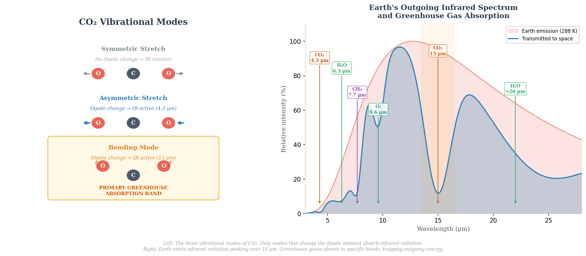
The greenhouse effect is often presented as a macroscopic phenomenon, a blanket of gas trapping heat, but its origin is molecular. A molecule absorbs infrared radiation only if the radiation's frequency matches a vibrational mode that produces a change in the molecule's electric dipole moment. Nitrogen (N₂) and oxygen (O₂), which together constitute 99 percent of the atmosphere, are symmetric diatomic molecules with no permanent dipole, and their vibrations produce no dipole change. They are therefore transparent to infrared radiation. Carbon dioxide, though it has no permanent dipole because its linear geometry makes the two carbon-oxygen dipoles cancel, possesses asymmetric vibrational modes that do produce a transient dipole. The asymmetric stretch, in which one oxygen moves closer to the carbon while the other moves away, and the bending modes, in which the molecule bends out of linearity, both generate oscillating dipoles that interact with infrared photons.
The bending mode of carbon dioxide absorbs most strongly at a wavelength of approximately 15 micrometres, which falls squarely within the thermal infrared spectrum that Earth's surface emits. This coincidence between the molecule's absorption frequency and the planet's emission spectrum is the physical basis of the greenhouse effect. Methane absorbs at different wavelengths, particularly around 3.3 and 7.7 micrometres, and its more complex geometry gives it more vibrational modes per molecule, which is why methane is a more potent greenhouse gas per molecule than carbon dioxide. Water vapour absorbs across a broad range of infrared wavelengths and is the most important greenhouse gas by total contribution, but its atmospheric concentration is controlled by temperature through evaporation and condensation, making it a feedback rather than a forcing agent. Carbon dioxide, by contrast, does not condense out of the atmosphere at any temperature Earth is likely to reach, making it the persistent, long-lived driver of the enhanced greenhouse effect.
Measuring Carbon: From Flask Networks to Satellites
The Architecture of Atmospheric Monitoring
Charles David Keeling's measurements at Mauna Loa established the principle that precise, continuous observations at well-chosen sites could reveal the behaviour of atmospheric carbon dioxide at the global scale. In the decades since, the monitoring infrastructure has expanded enormously, but the fundamental challenges Keeling faced remain central to the design of the global network. Atmospheric carbon dioxide varies in concentration with latitude, altitude, proximity to sources and sinks, time of day, season, and weather. Extracting a meaningful global signal from these variations requires not one observatory but a carefully designed network of stations, each sited to sample air that is representative of a large region rather than contaminated by local emissions.
The backbone of the current network is the Global Atmosphere Watch programme coordinated by the World Meteorological Organization, which integrates data from more than 50 stations spanning every continent and most ocean basins. Many of these stations use the flask sampling method pioneered by NOAA's Global Monitoring Laboratory, in which pairs of glass flasks are filled with ambient air at regular intervals and shipped to a central laboratory for analysis by gas chromatography and non-dispersive infrared spectroscopy. This approach ensures calibration against common reference standards, allowing measurements from stations in Alaska, Tasmania, the South Pole, and the Azores to be compared at the level of tenths of a part per million. Continuous in situ analysers, which measure carbon dioxide concentrations every few seconds, complement the flask network at key stations, capturing the short-term variability that flask sampling misses.
The network also measures other trace gases, including methane, nitrous oxide, sulphur hexafluoride (used as a tracer of atmospheric transport), and the stable isotope ratios of carbon dioxide. The δ¹³C measurements are particularly valuable because they distinguish between carbon sources: fossil fuel combustion and photosynthesis both deplete ¹³C relative to ¹²C, but by different amounts, and ocean exchange has its own isotopic signature. By combining concentration data with isotopic data from the same air samples, researchers can apportion observed changes in atmospheric carbon dioxide among fossil fuels, land biosphere exchange, and ocean exchange with a degree of precision that would be impossible from concentration measurements alone.
Satellite Remote Sensing and the View from Above
Ground-based stations, however numerous, provide point measurements. For a spatially continuous picture of carbon dioxide across the entire globe, satellite remote sensing is indispensable. The first dedicated carbon dioxide monitoring satellite, Japan's Greenhouse gases Observing SATellite (GOSAT), launched in 2009, demonstrated that space-based instruments could measure column-averaged carbon dioxide concentrations with sufficient precision to detect regional sources and sinks. NASA's Orbiting Carbon Observatory-2 (OCO-2), launched in 2014 after the loss of the original OCO during a launch failure in 2009, advanced this capability substantially, measuring reflected sunlight at wavelengths near 1.6 and 2.0 micrometres where carbon dioxide absorbs, and retrieving column-averaged CO₂ (designated XCO₂) with a precision of approximately 1 part per million.
The retrieval algorithm must account for the effects of atmospheric scattering by aerosols and thin clouds, variations in surface reflectance between ocean and land, and the temperature and pressure dependence of carbon dioxide absorption line shapes. These corrections require precise knowledge of the atmospheric state from meteorological analyses and from the satellite's own measurements at multiple wavelengths. The resulting column-averaged concentrations represent the mean carbon dioxide mixing ratio through the entire atmospheric column, weighted by pressure, which makes them more sensitive to near-surface concentrations where the atmosphere is densest and where the sources and sinks are located.
The power of satellite observations lies not in their absolute accuracy, which remains lower than that of ground-based instruments, but in their spatial coverage. OCO-2 collects roughly 100,000 observations per day across the sunlit hemisphere, mapping the global distribution of carbon dioxide at scales that reveal patterns invisible to the ground network. Satellite data have revealed, for example, the plumes of enhanced carbon dioxide downwind of major urban areas and industrial clusters, the seasonal drawdown of carbon dioxide over boreal forests in summer, and the outgassing of carbon dioxide from tropical oceans during El Nino events. The European Copernicus programme's CO2M satellites, under development in the mid-2020s, aim to provide the first space-based verification of national emissions inventories, a capability that would transform the transparency and accountability of international climate commitments.
Atmospheric Inversion Modelling
Neither ground stations nor satellites directly measure carbon fluxes, the flows of carbon between the atmosphere and the surface. They measure concentrations. Inferring fluxes from concentrations requires a technique called atmospheric inversion modelling, which uses observations of atmospheric carbon dioxide concentrations at many locations together with a model of atmospheric transport (wind patterns, turbulent mixing, convection) to work backward and estimate the surface fluxes that would produce the observed concentration field. The mathematical framework is Bayesian: prior estimates of surface fluxes, based on inventories and ecosystem models, are updated by the atmospheric observations to produce posterior flux estimates with quantified uncertainties.
Atmospheric inversions have become one of the most powerful tools in carbon cycle science. They revealed that the Northern Hemisphere land biosphere was a larger carbon sink than previously estimated, absorbing roughly 2 to 3 gigatonnes of carbon per year beyond what bottom-up ecosystem models predicted. They have tracked the weakening and recovery of the Southern Ocean carbon sink, detected the pulse of carbon released during major El Nino events, and provided independent verification of fossil fuel emission inventories at continental scales. The precision of inversion estimates is limited by the density of the observation network and by uncertainties in atmospheric transport models, but as satellite data become more abundant and transport models improve, inversions are converging toward a global carbon monitoring system capable of tracking fluxes at national and even sub-national scales in near-real time.
The Fast Carbon Cycle as a Coupled System
Photosynthetic Pathways and Their Carbon Cycle Implications
The overall equation of photosynthesis, 6CO₂ + 6H₂O → C₆H₁₂O₆ + 6O₂, conceals a diversity of biochemical strategies that plants have evolved to fix carbon under different environmental constraints. The ancestral and most widespread mechanism is the C3 pathway, named for the three-carbon molecule 3-phosphoglycerate that is the first stable product of carbon fixation by the enzyme RuBisCO (ribulose-1,5-bisphosphate carboxylase/oxygenase). C3 photosynthesis operates efficiently in cool, moist conditions with adequate carbon dioxide, and it dominates in forests, temperate grasslands, and most crop species including wheat, rice, and soybeans. However, RuBisCO has a well-known limitation: it also catalyses a competing reaction with oxygen, called photorespiration, which wastes fixed carbon and reduces the net efficiency of photosynthesis by 20 to 30 percent, particularly at high temperatures and low carbon dioxide concentrations.
The C4 pathway, evolved independently in more than 60 plant lineages, addresses this limitation through a spatial separation of initial carbon fixation and the Calvin cycle. In C4 plants, carbon dioxide is first fixed in mesophyll cells by the enzyme PEP carboxylase into a four-carbon compound (oxaloacetate), which is then shuttled to bundle-sheath cells where it releases carbon dioxide at high concentration directly to RuBisCO, effectively suppressing photorespiration. C4 plants, including maize, sugarcane, and many tropical grasses, are more efficient in hot, dry, high-light environments and have expanded their range during warm geological periods. The third strategy, CAM (Crassulacean Acid Metabolism), separates carbon fixation temporally rather than spatially: stomata open at night to take in carbon dioxide, which is stored as malic acid, and photosynthesis proceeds during the day with stomata closed, minimising water loss. CAM is characteristic of desert succulents and some epiphytes.
These distinctions matter for the carbon cycle because the relative abundance of C3 and C4 vegetation affects the magnitude and geographic distribution of terrestrial carbon uptake. Rising atmospheric carbon dioxide concentrations tend to favour C3 plants, which are carbon-limited under current conditions, through the carbon dioxide fertilisation effect. C4 plants, already operating at near-saturated carbon dioxide levels internally, benefit less. Models of future vegetation change under elevated carbon dioxide project shifts in the competitive balance between C3 and C4 species, with consequences for the strength and distribution of the terrestrial carbon sink that propagate through the entire budget equation.
Ocean-Atmosphere Gas Exchange and the Thin Boundary Layer
The exchange of carbon dioxide between the atmosphere and the ocean surface is governed by a remarkably thin layer of water. At the air-sea interface, a laminar boundary layer roughly 20 to 200 micrometres thick separates the turbulently mixed atmosphere from the turbulently mixed surface ocean. Molecular diffusion across this stagnant film is the rate-limiting step in gas exchange, and the thickness of the film depends primarily on wind speed: higher winds generate more turbulence, thin the film, and accelerate gas transfer. The gas transfer velocity k, typically expressed in centimetres per hour, scales approximately with the square of the wind speed at 10 metres above the surface, a relationship calibrated empirically from tracer experiments using deliberately released sulphur hexafluoride and helium-3 in the open ocean.
The net flux of carbon dioxide across the interface is proportional to the product of the gas transfer velocity and the difference in partial pressure of carbon dioxide between the atmosphere and the surface ocean, expressed as F = k · s · (pCO2,atm − pCO2,ocean), where s is the solubility coefficient. Regions where ocean pCO₂ is lower than atmospheric, typically cold high-latitude waters, are sinks; regions where ocean pCO₂ exceeds atmospheric, typically warm tropical upwelling zones, are sources. The net global flux is a sink of approximately 2.5 to 3 gigatonnes of carbon per year, but this net figure conceals enormous gross fluxes in both directions: roughly 80 gigatonnes of carbon per year entering the ocean and a slightly smaller amount leaving it, with the small residual representing the net anthropogenic uptake.
The Seasonal Breathing of the Planet
The Keeling Curve's annual sawtooth oscillation, with an amplitude of roughly 6 to 9 parts per million at Mauna Loa and even larger at higher northern latitudes, is one of the most vivid demonstrations that the biosphere is an active participant in the carbon cycle rather than a passive reservoir. The oscillation reflects the asymmetry of the Northern and Southern Hemispheres: approximately 65 percent of Earth's land surface lies north of the equator, and the great boreal and temperate forests of North America, Europe, and Asia drive a seasonal drawdown of atmospheric carbon dioxide each spring and summer that is only partially offset by the smaller Southern Hemisphere land mass during its growing season.
The pattern is not perfectly sinusoidal. The drawdown in spring and early summer is rapid, reflecting the explosive burst of photosynthetic activity as deciduous and boreal forests leaf out and grasslands green up across tens of millions of square kilometres within a few weeks. The rise through autumn and winter is more gradual, reflecting the slower and more continuous processes of decomposition and soil respiration that return carbon to the atmosphere. In the tropics, where vegetation is green year-round and the seasonal temperature variation is small, the atmospheric carbon dioxide oscillation is almost absent, typically less than 1 part per million. This latitudinal gradient in seasonal amplitude provides an independent confirmation that the oscillation is biologically driven: it tracks the geography of seasonal vegetation activity with remarkable fidelity.
The amplitude of this seasonal oscillation has been increasing over time. Measurements show that the peak-to-trough difference at Mauna Loa has grown by roughly 15 percent since the 1960s, and at high-latitude Arctic stations the increase is even larger. This amplification is attributed to a combination of factors: the carbon dioxide fertilisation effect enhancing summer photosynthesis, longer growing seasons as temperatures rise, and increased microbial respiration during warmer autumns and winters that amplifies the winter carbon dioxide peak. The Arctic stations record the largest seasonal swings because they are closest to the boreal forests that drive the oscillation, and because atmospheric mixing dilutes the signal as air moves toward the tropics. The growing seasonal amplitude is, in effect, the planet breathing more deeply as its metabolism accelerates under the influence of rising carbon dioxide and warming temperatures.
The Geological Carbon Cycle in Depth
Weathering Kinetics and the Walker Feedback
The self-regulating nature of Earth's climate over geological time depends on a negative feedback loop whose dynamics were formalised by James C. G. Walker, Paul Hays, and James Kasting in a landmark 1981 paper. Their insight was that the rate of chemical weathering of silicate rocks, which consumes atmospheric carbon dioxide, is temperature-dependent in a way that creates a thermostat. The temperature dependence arises through two pathways: directly, because the kinetics of mineral dissolution reactions follow the Arrhenius equation, with reaction rates approximately doubling for every 10-degree Celsius increase in temperature; and indirectly, because warmer temperatures drive more evaporation, more precipitation, and more runoff over exposed rock surfaces, all of which accelerate weathering.
The Walker feedback operates on timescales of hundreds of thousands to millions of years, far too slow to buffer the current human perturbation, but its existence explains why Earth has remained habitable despite enormous changes in solar luminosity and volcanic carbon dioxide output over four billion years. The mathematical framework developed by Robert Berner in the GEOCARB family of models extends this insight to reconstruct atmospheric carbon dioxide concentrations across the entire Phanerozoic Eon, the past 540 million years. GEOCARB models combine estimates of volcanic outgassing rates, continental configuration (which determines the area and latitude of exposed silicate rock), biological evolution (the spread of land plants, which accelerate weathering through root acids and soil formation), and ocean chemistry to produce carbon dioxide histories that agree broadly with proxy measurements from palaeosol carbonates, stomatal indices in fossil leaves, and boron isotope ratios in marine carbonates.
Snowball Earth and the Limits of the Thermostat
The geological record contains episodes that tested the carbonate-silicate thermostat to its limits and revealed both its power and its response time. The most dramatic of these are the Neoproterozoic glaciations, commonly known as "Snowball Earth" events, which occurred between approximately 720 and 635 million years ago. Geological evidence, including glacial deposits at palaeo-equatorial latitudes and the distinctive cap carbonate sequences that overlie them, suggests that Earth's surface may have been almost entirely covered by ice during at least two prolonged episodes, each lasting millions of years.
The Snowball Earth hypothesis, developed primarily by Joseph Kirschvink and elaborated by Paul Hoffman and Daniel Schrag, proposes that once ice cover extended to low latitudes, the ice-albedo feedback drove a runaway glaciation that the weathering thermostat could not immediately halt because ice-covered continents present no exposed silicate rock to weather. With weathering effectively shut down but volcanic outgassing continuing, carbon dioxide accumulated in the atmosphere over millions of years until concentrations reached levels estimated at 100 to 1,000 times the pre-industrial value. At that point, the extreme greenhouse warming was sufficient to begin melting the equatorial ice, and the ice-albedo feedback reversed, producing a rapid transition from icehouse to extreme greenhouse. The cap carbonates, thick layers of calcium carbonate deposited in the aftermath, record the intense chemical weathering that ensued as the thermostat finally engaged under extreme carbon dioxide conditions, drawing the gas back down and restoring a temperate climate.
These events demonstrate that the thermostat works, but on its own timescale. It can recover the planet from the most extreme perturbations the geological record has to offer, but the recovery takes millions of years, and the intervening conditions are catastrophically outside the range compatible with complex life as it exists today. The Snowball Earth episodes are relevant to the modern carbon perturbation not as a direct analogue, since the mechanisms differ entirely, but as a demonstration of what happens when the carbon cycle is pushed far from equilibrium: the system eventually returns, but the return time is measured in millions of years, and the transitional states can be lethal to existing ecosystems. The current anthropogenic carbon injection is unique in the geological record for its speed, and the question of whether natural self-regulation can operate fast enough to prevent dangerous overshoot is one that the geological precedents answer with a sobering clarity: it cannot, not on any timescale relevant to the civilisation that created the perturbation.
Organic Carbon Burial and the Oxygen Connection
The geological carbon cycle has a second major pathway for removing carbon from the atmosphere: the burial of organic carbon in sediments. When organisms die and their remains are deposited in environments where decomposition is incomplete, typically in anoxic marine basins or waterlogged soils, the organic carbon is preserved and eventually lithified into carbon-rich rocks such as black shales, coal, and oil source rocks. This burial removes carbon from the active cycle for geological timescales and has a profound additional consequence: because photosynthesis produces oxygen as a by-product, and the burial of organic carbon prevents that carbon from being re-oxidised (which would consume oxygen), the net effect of organic carbon burial is an increase in atmospheric oxygen.
The relationship between organic carbon burial and atmospheric oxygen links the carbon cycle to the history of life in a deep and beautiful way. The Great Oxidation Event, roughly 2.4 billion years ago, was driven in part by the sustained burial of organic carbon produced by cyanobacterial photosynthesis, which allowed free oxygen to accumulate in the atmosphere for the first time. The Carboniferous coal forests buried vast quantities of organic carbon over roughly 60 million years, and atmospheric oxygen during this period is estimated to have reached 30 to 35 percent, compared to 21 percent today, enabling the giant insects and amphibians that characterise Carboniferous fauna. The carbon now being extracted from those same coal deposits and burned is, in a precise chemical sense, reversing the oxygen-carbon transaction that the Carboniferous biosphere conducted over tens of millions of years.
The Carbon Budget, Ocean Chemistry, and Sink Dynamics
The Revelle Factor and Ocean Buffering Capacity
The ocean's ability to absorb carbon dioxide from the atmosphere is not unlimited, and the chemical reason is captured by a single quantity: the Revelle factor, also called the buffer factor. When carbon dioxide dissolves in seawater, it enters a system of chemical equilibria involving dissolved CO₂, carbonic acid, bicarbonate ions, and carbonate ions. The total quantity of all these species is called dissolved inorganic carbon (DIC). If the ocean were a simple solution with no buffering chemistry, a given percentage increase in atmospheric carbon dioxide would produce an equal percentage increase in dissolved carbon dioxide, and from there an equal percentage increase in DIC. The buffering chemistry of seawater prevents this proportional response: because bicarbonate and carbonate ions react with the incoming carbon dioxide, the system absorbs much of the perturbation without a proportional rise in dissolved CO₂.
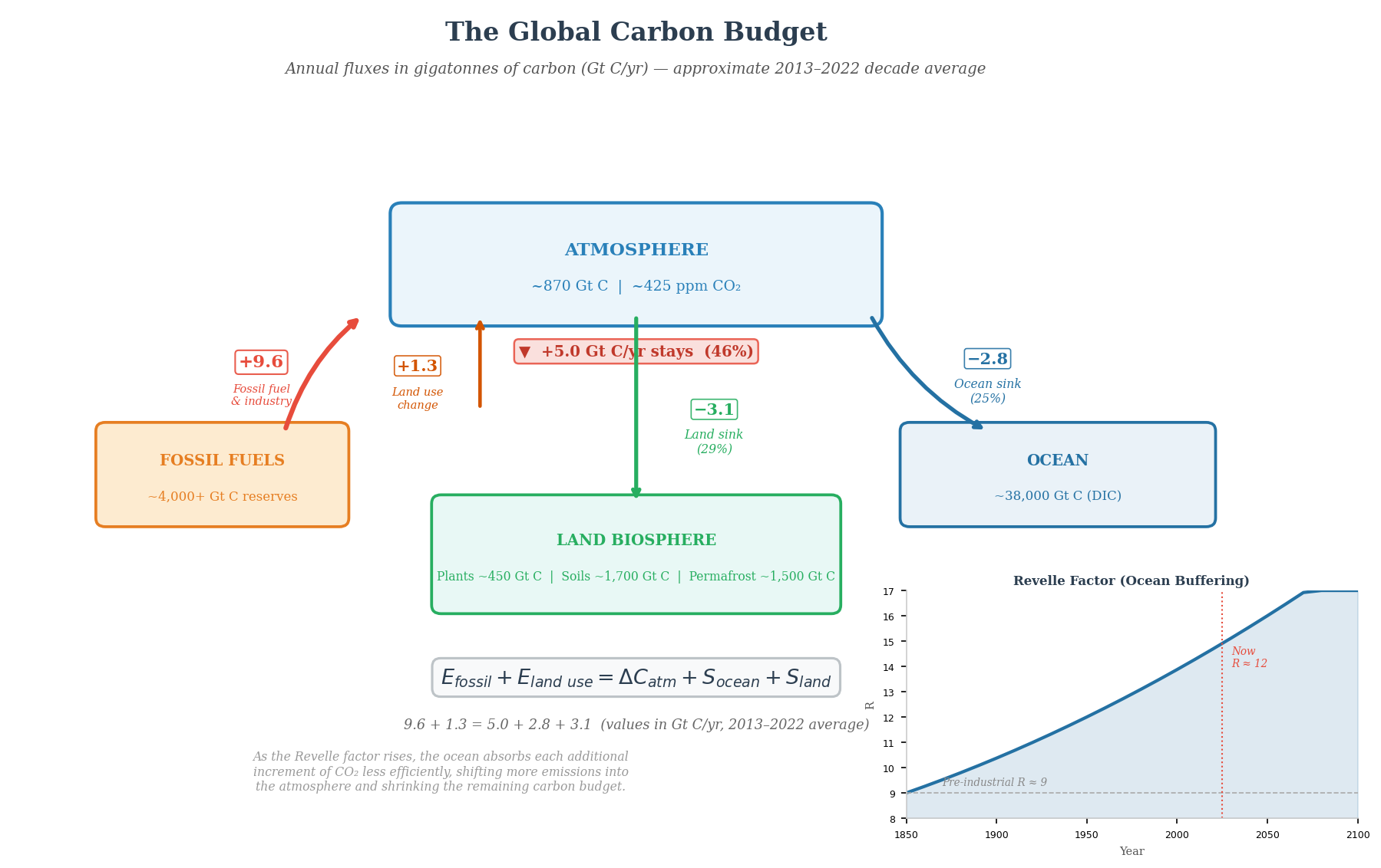
The Revelle factor R quantifies the departure from proportional response. It is defined as the ratio of the fractional change in ocean surface pCO₂ to the fractional change in DIC: R = (Δ pCO₂ / pCO₂) / (Δ DIC / DIC). In pre-industrial surface seawater, R was approximately 9, meaning that a 1 percent increase in DIC produced a 9 percent increase in surface pCO₂. As the ocean absorbs more anthropogenic carbon dioxide and DIC increases, the buffering capacity of the carbonate system is progressively consumed. The carbonate ion concentration decreases because carbonate reacts with the incoming carbon dioxide to form bicarbonate, and the Revelle factor rises. In many ocean regions today, R exceeds 12, and under high-emission scenarios it is projected to exceed 15 by the end of the century. A higher Revelle factor means the ocean's chemical capacity to absorb additional carbon dioxide without a large increase in surface pCO₂ is diminishing.
This progressive reduction in buffering capacity has a direct consequence for the airborne fraction. As the ocean becomes less efficient at absorbing each additional increment of carbon dioxide, a larger fraction of each year's emissions remains in the atmosphere. The ocean has not stopped absorbing carbon, and in absolute terms it continues to take up more each year as the atmospheric concentration rises, but its efficiency per unit of emission is declining. This is one of the mechanisms that could cause the airborne fraction to increase over the coming decades, accelerating the accumulation of carbon dioxide in the atmosphere even if annual emissions remain constant.
The Biological Pump: Efficiency and Vulnerability
The biological pump transfers organic carbon from the sunlit surface ocean, where it interacts with the atmosphere, to the deep ocean, where it is sequestered for centuries to millennia. The pump's efficiency depends on a chain of biological and physical factors: the rate of primary production by phytoplankton in the euphotic zone, the fraction of that production that is exported below the mixed layer as sinking particles rather than being remineralised (consumed by bacteria and zooplankton) in the surface, and the depth at which the sinking particles are eventually decomposed and their carbon released as dissolved inorganic carbon.
The export ratio, the fraction of surface production that sinks below 100 metres, varies from less than 5 percent in nutrient-poor subtropical gyres to more than 30 percent in productive high-latitude and upwelling regions. The composition of the phytoplankton community strongly influences this ratio: diatoms, large silica-shelled algae that dominate in nutrient-rich waters, produce heavy, fast-sinking particles that efficiently export carbon, while smaller cyanobacteria and picoplankton are more likely to be recycled within the surface layer. Ocean warming and increased stratification favour smaller phytoplankton by reducing nutrient supply from below, which could shift community composition in a direction that weakens the biological pump.
The remineralisation depth, the average depth at which sinking organic carbon is decomposed, determines how long the exported carbon is isolated from the atmosphere. If carbon is remineralised at 200 metres, it may return to the surface within decades through mixing and upwelling. If it reaches 1,000 metres or below, it enters deep water masses that circulate on timescales of centuries to millennia before resurfacing. Climate models project that warming will both reduce export production and shift remineralisation toward shallower depths, a combination that would weaken the biological pump's contribution to carbon sequestration. The magnitude of this weakening remains uncertain, but it represents one of several pathways by which the ocean carbon sink could lose efficiency as the climate warms.
Partitioning Emissions: Atmosphere, Land, and Ocean
The carbon budget equation, Eff + Eluc = ΔCatm + Socean + Sland + Bim, is the master accounting identity of climate science, where Eff represents fossil fuel and industrial emissions, Eluc represents land use change emissions, ΔCatm is the atmospheric growth rate, Socean and Sland are the ocean and land sinks, and Bim is the budget imbalance, a residual term that captures the mismatch between independently estimated sources and sinks. The Global Carbon Project, which publishes the definitive annual assessment of this budget, estimates each term using different methods: fossil fuel emissions from energy statistics and trade data, land use change emissions from satellite-observed deforestation combined with bookkeeping models, atmospheric growth from the global monitoring network, ocean uptake from ocean biogeochemical models constrained by ship-based measurements, and land uptake as the residual that balances the equation.
The budget imbalance term deserves attention because it quantifies how well the independent estimates of sources and sinks actually close the budget. In the most recent decade, this imbalance has averaged roughly 0.3 gigatonnes of carbon per year, a residual that reflects measurement uncertainty in all the other terms rather than a missing flux. The fact that the imbalance is small relative to the total fluxes provides confidence that the budget is understood at the first-order level, even as the second-order details of regional and interannual variability remain areas of active investigation.
The three-way partition of emissions among atmosphere, ocean, and land has been remarkably consistent over recent decades at roughly 45, 25, and 30 percent respectively, but this apparent stability conceals important trends. The absolute magnitude of each sink has grown, absorbing more carbon each year as emissions have risen, but the ocean sink's efficiency, measured as the fraction of emissions absorbed, has shown signs of decline in some analyses. The land sink is highly variable from year to year, driven by climate fluctuations such as El Nino, which suppresses tropical vegetation growth and shifts the land from net sink toward net source. In the strong El Nino year of 2015 to 2016, the atmospheric growth rate spiked to 3.4 parts per million per year, well above the long-term average, almost entirely because the land sink weakened while emissions held roughly steady.
The Carbon Dioxide Fertilisation Effect and Its Limits
The land sink owes a significant fraction of its current magnitude to the carbon dioxide fertilisation effect: the enhancement of photosynthesis that occurs when plants are exposed to higher atmospheric carbon dioxide concentrations. Because carbon dioxide is a substrate for RuBisCO, higher concentrations increase the rate of carbon fixation, particularly in C3 plants. Free-Air CO₂ Enrichment (FACE) experiments, in which circular arrays of pipes release carbon dioxide around forest plots or crop fields to elevate local concentrations to levels expected later this century, have confirmed that elevated carbon dioxide increases plant growth, but the magnitude and sustainability of the response depend heavily on other factors.
Nitrogen limitation is the most widely documented constraint. Forests growing on nitrogen-poor soils show little sustained growth response to elevated carbon dioxide because nitrogen is required for the proteins and enzymes that support increased photosynthesis. Phosphorus limitation is similarly important in tropical forests on ancient, weathered soils. Water availability interacts with the fertilisation effect in complex ways: elevated carbon dioxide allows plants to partially close their stomata while maintaining photosynthetic rates, reducing water loss per unit of carbon fixed and potentially increasing drought tolerance, but this benefit has limits in severely water-stressed conditions. The longest-running FACE experiments, now extending beyond 15 years, suggest that the initial growth enhancement diminishes over time as nutrient limitation constrains the capacity of ecosystems to capitalise on the additional carbon dioxide. The implication for the carbon budget is that the land sink's growth in response to rising emissions may slow or saturate, increasing the airborne fraction and accelerating atmospheric accumulation.
Residence Times, Committed Warming, and the Budget Clock
The Multi-Timescale Removal of Atmospheric Carbon Dioxide
A common misconception about carbon dioxide is that it has a single atmospheric lifetime analogous to the approximately 12-year lifetime of methane. In reality, the removal of a pulse of carbon dioxide from the atmosphere follows a distribution of timescales governed by distinct physical and chemical processes. Within the first decade, roughly 25 to 30 percent of the pulse is absorbed by the surface ocean and the land biosphere, processes that operate on timescales of years. Over the following century, an additional 20 to 25 percent is taken up as the ocean's surface layer equilibrates more fully with the deep ocean through thermohaline circulation. On timescales of one to ten thousand years, ocean mixing and calcium carbonate dissolution from marine sediments, a process called carbonate compensation, remove most of the remaining excess. But even after 100,000 years, approximately 7 to 8 percent of the original pulse persists in the atmosphere, removable only by the silicate weathering feedback operating on geological timescales.
This multi-timescale removal has a consequence that is both mathematically precise and practically sobering: the warming caused by a given quantity of carbon dioxide emissions is effectively permanent on any timescale relevant to human civilisation. The IPCC has formalised this insight as the approximately linear relationship between cumulative carbon dioxide emissions and peak warming, a relationship known as the transient climate response to cumulative emissions (TCRE). The TCRE is estimated at approximately 1.65 degrees Celsius per 1,000 gigatonnes of carbon dioxide emitted, with a likely range of 1.0 to 2.3 degrees per 1,000 gigatonnes. This linearity, which arises from a near-cancellation between the logarithmic saturation of carbon dioxide's radiative forcing and the declining efficiency of ocean carbon uptake, means that every tonne of carbon dioxide emitted contributes roughly the same increment of eventual warming regardless of when it is emitted or the current concentration.
The Remaining Carbon Budget and Its Uncertainties
The TCRE framework provides the scientific basis for the remaining carbon budget: the total quantity of carbon dioxide that can still be emitted while limiting global warming to a specified temperature target with a specified probability. The IPCC's Sixth Assessment Report estimated that from the beginning of 2020, the remaining carbon budget for limiting warming to 1.5 degrees Celsius with a 50 percent probability was approximately 500 gigatonnes of carbon dioxide, and for 2 degrees with a 67 percent probability approximately 1,150 gigatonnes. At the 2023 global emission rate of approximately 40 gigatonnes of carbon dioxide per year from all sources, the 1.5-degree budget provides roughly a decade of emissions at current rates, and the 2-degree budget roughly three decades.
These budgets carry substantial uncertainties that cut in both directions. On the side of larger budgets, some analyses suggest that natural sinks may continue to strengthen and absorb a growing share of emissions. On the side of smaller budgets, permafrost carbon feedbacks, which are not fully represented in the models used to calculate TCRE, would add additional warming for any given level of human emissions, effectively reducing the remaining budget. The uncertainty in Earth system feedbacks, the uncertainty in historical warming (which determines how much budget has already been spent), and the contributions of non-carbon-dioxide greenhouse gases all introduce ranges of hundreds of gigatonnes around the central estimates. The most consequential uncertainty, however, is not scientific but political: whether the global economy will actually achieve the emission reductions implied by these budgets, given that no major economy has yet demonstrated sustained reductions at the required pace.
Equity, Accountability, and the Distribution of Carbon Space
The remaining carbon budget is a finite physical quantity that must be shared among nearly eight billion people across nations at vastly different levels of economic development. The historical dimension of this challenge is stark. The United States, with roughly four percent of the world's population, has contributed approximately 25 percent of all cumulative carbon dioxide emissions since the onset of industrialisation. The European Union adds another 17 percent. Together, these wealthy nations have consumed roughly half of the total carbon budget ever available, building their prosperity on a resource, atmospheric space for carbon dioxide, that they now propose to ration. India, with 18 percent of the world's population, has contributed approximately 3 percent of cumulative emissions. Sub-Saharan Africa, with more than 14 percent of the global population, has contributed less than 4 percent.
The principle of common but differentiated responsibilities, enshrined in the United Nations Framework Convention on Climate Change, acknowledges this asymmetry but does not resolve it. The remaining carbon budget is shrinking rapidly, and the countries that have used the least of the historical budget are the ones that most urgently need energy-intensive development, including electrification, industrialisation, and infrastructure construction, to lift their populations out of poverty. The tension between the physical constraint of the budget and the moral imperative of equitable development defines the central political challenge of climate policy. Consumption-based accounting, which assigns emissions to the consumers of goods rather than their producers, reveals additional layers of inequity: wealthy nations that have offshored their manufacturing to developing countries appear cleaner in territorial inventories but carry larger footprints when the emissions embedded in their imports are counted. The carbon budget is a scientific quantity, but its distribution is an ethical and political question that science can inform but cannot resolve.
The architecture of carbon science assembled in the preceding sections, from molecular vibrations to satellite remote sensing, from the Revelle factor's declining buffering to the shrinking carbon budget, provides the quantitative foundation on which the rest of carbon science rests.