A supervised learning framework can be built from first principles: data as feature vectors and labels, models as parameterised functions, loss functions as the definition of what "wrong" means, and gradient descent as the engine that drives parameters toward low loss. The core tools — linear regression, logistic regression, the mean squared error, the cross-entropy loss, the gradient update rule — are clean, mathematically transparent, and provably optimal for a specific class of problems. They are also, for a wide and important range of real-world tasks, not enough.
The limitation is not a matter of training procedure or data quantity. It is structural. A linear model can only separate classes with a flat boundary, and it can only learn relationships that are additive combinations of the input features. When the true pattern in the data is curved, or when the relevant information is encoded in interactions among features rather than in the features themselves, no amount of gradient descent will rescue a linear model from systematic failure. Understanding exactly where this failure occurs — and what it takes to overcome it — is the first step toward neural networks.
This material fills the conceptual space between linear models and multi-layer networks. It begins with the concrete failures of linearity and proceeds through the probabilistic foundations that connect loss functions to statistical reasoning, the practical refinements that make gradient-based optimisation workable on complex landscapes, the model selection machinery that guards against overfitting, and the non-neural learning algorithms that dominated applied machine learning for decades before deep learning eclipsed them. It ends with a question: what happens when the model is allowed to learn its own features?
The Limits of Linearity
When a Straight Line Cannot Separate
The logistic regression classifier makes its predictions by computing a weighted sum of the input features, adding a bias, and passing the result through a sigmoid. Its decision boundary — the set of points in feature space where the predicted probability is exactly 0.5 — is defined by wtop x + b = 0, which is a hyperplane. In two dimensions, this is a straight line. In three dimensions, it is a flat plane. In any number of dimensions, it is a flat surface that divides the feature space into two half-spaces.
This works remarkably well when the two classes are, in fact, separable by such a surface. A dataset of tumours described by size and cell-density might be cleanly divided into benign and malignant by a single straight cut through the feature plane. A collection of emails described by the frequency of a handful of suspicious words might be separated from legitimate mail by a hyperplane in word-frequency space. For problems where the class boundary is roughly linear, logistic regression is fast, interpretable, and hard to beat.
The trouble begins when the boundary is not linear. Consider a dataset where the positive examples cluster in a ring around the origin in two-dimensional space, and the negative examples occupy the centre. No straight line can separate the ring from the centre — any line that correctly classifies points on one side of the ring will misclassify points on the other side. A logistic regression model trained on this data will converge to the best linear approximation of the true boundary, which is a compromise that misclassifies a substantial fraction of both classes. The model is not undertrained; it is structurally incapable of solving the problem. The hypothesis class — the set of all linear functions — does not contain any function that correctly separates the two classes.
This failure is not an edge case. Many important classification problems involve class boundaries that curve, wrap, or fragment across the feature space. Medical diagnosis, image recognition, speech classification, and natural-language understanding all involve decision surfaces of a complexity that no hyperplane can approximate. The question that follows from this observation is precise: what is the simplest problem that a linear classifier cannot solve, and what does that failure reveal about the kind of model that is needed?
The XOR Problem and Its Lessons
The most famous demonstration of the limits of linear classification is the XOR problem, and its significance in the history of machine learning is difficult to overstate. XOR, short for "exclusive or," is a Boolean function of two binary inputs: it returns 1 when exactly one of the two inputs is 1, and 0 otherwise. The four input-output pairs are (0,0) → 0, (0,1) → 1, (1,0) → 1, and (1,1) → 0.
Plotted as points in two-dimensional space, the four inputs form the corners of a unit square. The two positive examples sit at (0,1) and (1,0) — opposite corners — and the two negative examples sit at (0,0) and (1,1) — the other pair of opposite corners. No straight line can separate the positive corners from the negative corners, because the positive points are not on the same side of any line through the plane. This is easy to verify geometrically: any line that puts (0,1) and (1,0) on one side must also include either (0,0) or (1,1), or both, on that same side.
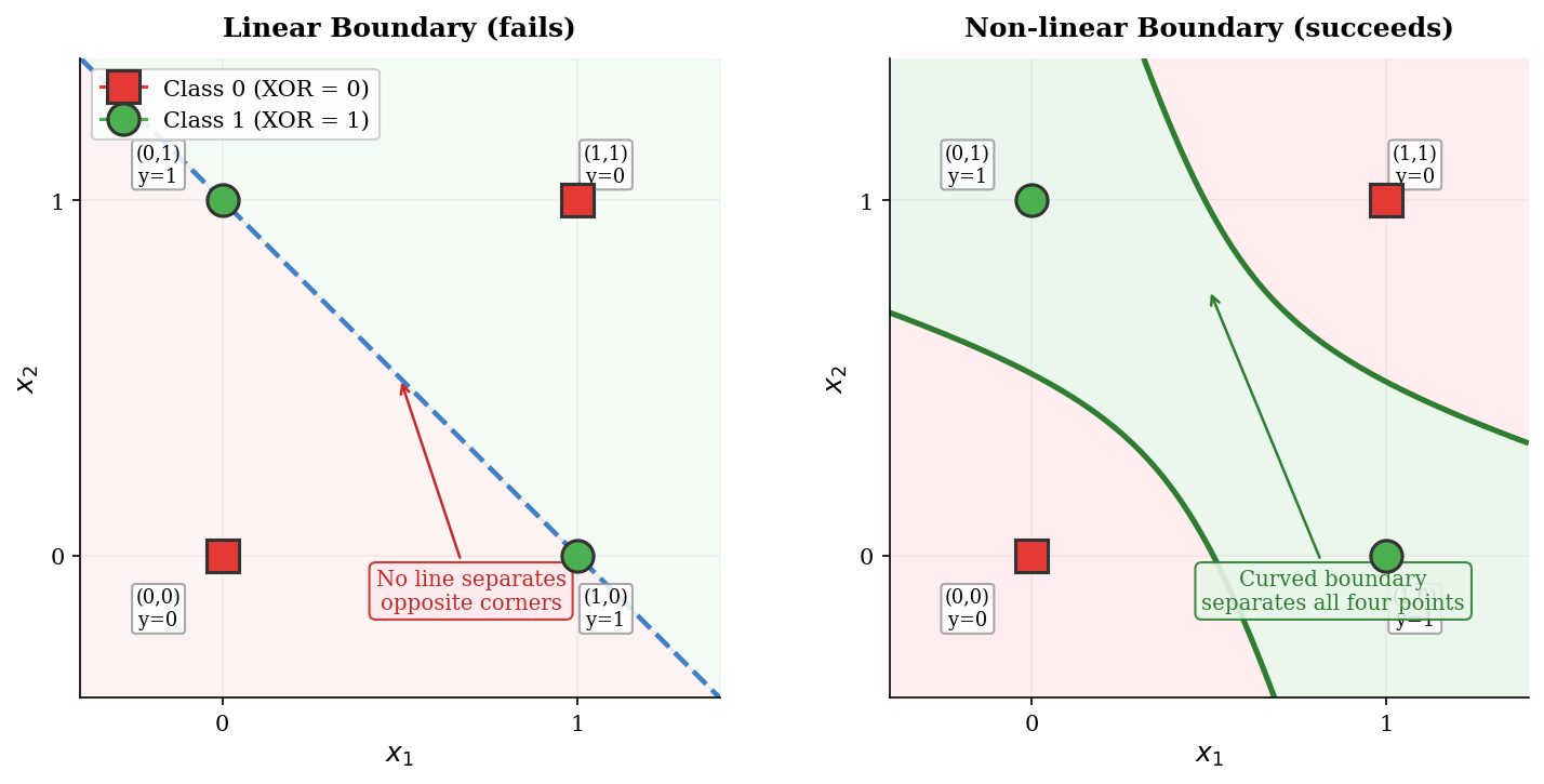
Minsky and Papert's 1969 book "Perceptrons" proved this result rigorously and extended it to a broader class of problems that single-layer networks cannot solve. The impact was devastating: it contributed directly to the first AI winter, a period of reduced funding and interest in neural network research that lasted through much of the 1970s. The irony is that the solution was already known in principle. Two linear classifiers, arranged in sequence, can solve XOR: the first classifier computes an intermediate feature that transforms the geometry of the problem, and the second classifier draws a linear boundary in the transformed space. This is exactly what a two-layer neural network does. But in 1969, nobody had an efficient algorithm for training the weights of both layers simultaneously, and the theoretical impossibility result for single layers overshadowed the theoretical possibility for multiple layers.
The XOR problem is important not because exclusive-or is a useful function in itself, but because it is the simplest possible illustration of a general phenomenon: nonlinear structure in data requires nonlinear models. The four-point XOR dataset makes this visible in a way that larger, messier datasets do not. Every time a practitioner encounters a classification problem where classes interleave, where clusters overlap in original feature space, or where the relevant pattern involves an interaction between features rather than a single feature acting alone, the same fundamental issue is at work.
Polynomial Features and the Complexity Trade-Off
One response to the failure of linearity is to remain within the linear framework but enrich the input representation. If the original features are x₁ and x₂, a linear model can only learn boundaries of the form w₁ x₁ + w₂ x₂ + b = 0. But if we create new features by computing products and powers of the originals — x₁², x₂², x₁ x₂, and perhaps higher-order terms — and include these as additional inputs, a linear model in the expanded feature space corresponds to a polynomial boundary in the original space. The boundary w₁ x₁ + w₂ x₂ + w₃ x₁² + w₄ x₂² + w₅ x₁ x₂ + b = 0 is a conic section — an ellipse, hyperbola, or parabola — which can separate classes that no straight line can.
This technique, called polynomial feature expansion, is genuinely useful for small and moderate-dimensional problems. Adding quadratic features to the XOR problem, for instance, makes it linearly separable in the expanded space: the feature x₁ x₂ takes value 0 for the positive examples (0,1) and (1,0) and value 0 or 1 for the negative examples, which is enough to separate them with a hyperplane that includes the interaction term.
The difficulty is that the number of polynomial features grows combinatorially with the degree and the number of original features. For d original features and polynomial degree p, the number of terms is C(d+p, p), which for d = 100 and p = 3 is over 176,000. For d = 1000 — the scale of a modest image or text representation — a cubic expansion produces hundreds of millions of features, most of which are uninformative noise. The model must estimate a weight for each of these features from a finite training set, and the more parameters the model has relative to the number of training examples, the greater the risk of overfitting. Polynomial expansion trades one problem (insufficient model complexity) for another (excessive model complexity and computational cost).
This trade-off hints at a deeper question: is there a way to introduce nonlinearity without manually specifying which nonlinear combinations of features to use? A method that discovers the right nonlinear features from the data itself, rather than requiring a human to enumerate them? The answer is yes, and it is precisely what neural networks achieve through learned hidden representations. But before arriving at that answer, there is value in understanding the statistical and optimisation foundations that make learning possible at all.
Probability, Bayes, and the Statistical View of Learning
Probability as the Language of Uncertainty
Machine learning operates in a world of uncertainty. The data is noisy, the features are incomplete, the labels may contain errors, and the true relationship between inputs and outputs is unknown. Probability theory provides the formal language for reasoning under these conditions, and understanding this language illuminates why the loss functions and training procedures used throughout this material take the forms they do.
A probability distribution assigns a number between 0 and 1 to each possible outcome, with the constraint that the probabilities of all possible outcomes sum to 1. For a discrete random variable X that can take values x₁, x₂, …, xₖ, the probability mass function P(X = xᵢ) specifies the probability of each value. For a continuous random variable, the probability density function p(x) specifies the relative likelihood of values, with the constraint that ∫ p(x) dx = 1. Probabilities can be conditional: P(Y = y | X = x) is the probability that Y takes value y given that X has been observed to take value x. The joint probability P(X = x, Y = y) factors as P(Y = y | X = x) · P(X = x), relating the joint distribution to the conditional and marginal distributions.
In the supervised learning context, the training data consists of pairs (x⁽ⁱ⁾, y⁽ⁱ⁾) drawn from some unknown joint distribution P(X, Y). The model's task is to approximate the conditional distribution P(Y | X) — the probability of the label given the features. A classifier that outputs P(Y = 1 | x) = 0.87 is not merely predicting a class; it is expressing a degree of belief, calibrated by the training data, about what the true label is likely to be. This probabilistic framing connects machine learning to centuries of statistical theory and provides principled answers to questions about what loss functions to use, how to combine prior knowledge with observed data, and how to quantify the uncertainty in predictions.
Bayes' Theorem and Prior Knowledge
The central theorem of probabilistic reasoning is Bayes' theorem, which describes how to update a belief in light of new evidence:
Here H is a hypothesis and D is observed data. The term P(H) is the prior probability — the degree of belief in the hypothesis before seeing the data. The term P(D | H) is the likelihood — the probability of observing the data if the hypothesis were true. The term P(H | D) is the posterior probability — the updated belief after seeing the data. The denominator P(D) is the evidence, a normalising constant that ensures the posterior probabilities sum to 1.
In a machine learning setting, the hypothesis is a set of model parameters θ, and the data D is the training set. Bayes' theorem then reads:
The prior P(θ) encodes assumptions about the parameters before any data is seen — for instance, a preference for small parameter values, which corresponds to a belief that simpler models are more likely to be correct. The likelihood P(D | θ) is the probability of the training data under the model with parameters θ. The posterior P(θ | D) is the distribution over parameters after learning from the data.
A concrete example makes the machinery tangible. Suppose you are building a spam filter and you have a prior belief that the weight on any particular word should be close to zero — most words, after all, are irrelevant to spamminess. This belief is the prior P(θ). You then observe 10,000 labelled emails and compute how likely that data would be under various weight settings — the likelihood P(D | θ). The posterior combines these: if a word like "lottery" appears overwhelmingly in spam emails, the likelihood will overpower the prior and assign a large positive weight. If a word like "the" appears equally in both classes, the likelihood is nearly flat with respect to its weight, and the prior pulls the weight back toward zero. The posterior thus reflects a compromise between what you assumed before seeing data and what the data actually shows.
Full Bayesian inference — computing the entire posterior distribution and using it to make predictions by averaging over all possible parameter values — is computationally intractable for all but the simplest models. The posterior is typically a complex, high-dimensional distribution with no closed-form expression. But the Bayesian framework provides the conceptual foundation for many practical techniques: regularisation can be understood as encoding a prior preference for simple models, ensemble methods approximate Bayesian model averaging, and the bias-variance trade-off has a natural Bayesian interpretation in terms of the width and location of the posterior.
Maximum Likelihood: Where Loss Functions Come From
The most common practical simplification of Bayesian inference is maximum likelihood estimation (MLE), which replaces the full posterior with a single point estimate: the parameter values that maximise the likelihood P(D | θ).
For a dataset of n independent examples, the likelihood is the product of the probabilities assigned to each example:
Maximising this product is equivalent to maximising its logarithm (since the logarithm is monotonically increasing), and maximising the log-likelihood is equivalent to minimising the negative log-likelihood:
This expression should look familiar. For a logistic regression model where P(Y = 1 | x; θ) = ŷ and P(Y = 0 | x; θ) = 1 - ŷ, the negative log-likelihood of a single example is -[y log ŷ + (1-y) log(1-ŷ)], which is exactly the binary cross-entropy loss. For a linear regression model where the label is assumed to follow a Gaussian distribution centred on the prediction — y ~ 𝒩(f(x; θ), σ²) — the negative log-likelihood, up to a constant, is proportional to (y - ŷ)², which is the mean squared error.
The loss functions are therefore not arbitrary choices. They are the negative log-likelihoods corresponding to specific probabilistic assumptions about how labels are generated. Cross-entropy loss assumes that labels are drawn from a Bernoulli distribution parameterised by the model's output. Mean squared error assumes that labels are drawn from a Gaussian distribution centred on the model's prediction. This connection reveals that minimising a loss function is equivalent to finding the most likely parameters under a specific statistical model of the data — a result that grounds the entire training procedure in probability theory.
Optimisation in Practice
Beyond Vanilla Gradient Descent: Momentum
The gradient descent update rule — θ ← θ - η ∇θ ℒ — is the conceptual foundation of training, but its behaviour on real loss landscapes is often poor. The difficulty arises when the loss surface is not equally curved in all directions: steep in some parameter directions and shallow in others. On such surfaces, vanilla gradient descent oscillates rapidly in the steep directions (where the gradient is large) while making slow progress in the shallow directions (where the gradient is small). The path to the minimum resembles a ball bouncing back and forth across a narrow ravine rather than rolling smoothly down to the bottom.
Momentum addresses this by adding inertia to the optimisation process. Instead of updating the parameters using only the current gradient, the algorithm maintains a running average of past gradients — a velocity vector — and uses that velocity to determine the update direction:
The hyperparameter β (typically 0.9) controls how much of the previous velocity is retained. When the gradient consistently points in the same direction across successive steps, the velocity accumulates and the effective step size grows — the optimiser accelerates in that direction. When the gradient oscillates, successive gradients partially cancel in the velocity, damping the oscillation. The physical analogy is a heavy ball rolling down a surface: it builds speed on consistent downhill slopes and resists sudden changes in direction.
Momentum was introduced by Polyak in 1964 and remains a component of virtually every modern optimisation algorithm used in deep learning. Its effect is particularly pronounced on the elongated, ravine-like loss surfaces that arise in training neural networks, where it can reduce the number of iterations required for convergence by an order of magnitude compared to vanilla gradient descent.
Adaptive Learning Rates and the Adam Optimiser
Momentum solves the oscillation problem but uses the same learning rate η for every parameter. In a neural network with millions of parameters, the optimal step size can vary enormously from one parameter to another: parameters connected to frequently activated features may need small steps to avoid overshooting, while parameters connected to rare features may need large steps to make progress before training ends.
Adaptive learning rate methods address this by maintaining a separate effective learning rate for each parameter, adjusted automatically based on the history of gradients for that parameter. The AdaGrad algorithm (Duchi, Hazan, and Singer, 2011) divides each parameter's learning rate by the square root of the sum of all its past squared gradients, giving a larger effective learning rate to parameters that have historically received small gradients and a smaller rate to those that have received large gradients. The RMSProp algorithm (Hinton, unpublished lecture notes, 2012) modifies this by using an exponentially weighted moving average of squared gradients instead of a cumulative sum, preventing the effective learning rate from decaying to zero as training progresses.
The Adam optimiser (Kingma and Ba, 2015) combines momentum with adaptive learning rates, maintaining both a first-moment estimate mₜ (the exponential moving average of gradients, analogous to momentum) and a second-moment estimate vₜ (the exponential moving average of squared gradients, analogous to RMSProp). The update rule is:
where m̂ₜ and v̂ₜ are bias-corrected versions of the moment estimates (necessary because the estimates are biased toward zero in the early iterations), and ε is a small constant (typically 10⁻⁸) that prevents division by zero. The default hyperparameters β₁ = 0.9, β₂ = 0.999, and η = 0.001 work well across a remarkably wide range of problems, which is a large part of Adam's appeal. It has been the default optimiser for most deep learning research since its introduction.
Local Minima, Saddle Points, and the Loss Landscape
For linear models, the loss landscape is convex: there is a single global minimum, and gradient descent is guaranteed to find it. For neural networks, the loss landscape is profoundly non-convex, with a complex topology that includes multiple local minima, saddle points, and flat plateaus. Understanding this landscape is essential for understanding why training neural networks works at all.
A local minimum is a point where the loss is lower than at all nearby points but not necessarily the lowest anywhere on the landscape. Early theoretical concerns about neural network training focused on the danger of gradient descent becoming trapped in poor local minima — valleys that are far above the global minimum in loss. If training routinely converged to such valleys, neural networks would be unreliable and their performance would depend sensitively on the random initialisation of parameters.
In practice, this concern has turned out to be less severe than originally feared, particularly for large networks. Empirical and theoretical work by Dauphin, Pascanu, Gulcehre, Cho, Ganguli, and Bengio (2014) showed that in high-dimensional loss landscapes, most critical points — points where the gradient is zero — are not local minima but saddle points: points where the loss curves upward in some directions and downward in others. A random critical point in a d-dimensional landscape is a local minimum only if the loss curves upward in all d directions simultaneously, which becomes exponentially unlikely as d grows. For a network with millions of parameters, nearly all critical points are saddle points, and gradient descent can escape them by following the downward-curving directions.
Furthermore, Choromanska, Henaff, Mathieu, Arous, and LeCun (2015) provided evidence that in large networks, the local minima that do exist tend to have loss values close to the global minimum. The practical implication is that for sufficiently large networks, most local minima are "good enough," and the choice between them matters less than the choice of architecture, data, and regularisation.
Model Selection and Validation
Cross-Validation: Using Data Wisely
The train-test split is the basic tool for evaluating generalisation. The test set provides an unbiased estimate of performance on new data, but it serves this purpose only if it is used once — after all modelling decisions have been finalised. The validation set, a second holdout used during development, is where model selection happens. But carving a dataset into three pieces — training, validation, and test — reduces the amount of data available for training, which is particularly costly when the dataset is small.
Cross-validation is a technique that addresses this tension by using the same data for both training and validation, but never at the same time. The most common form is k-fold cross-validation. The training data is divided into k roughly equal subsets, or folds. The model is trained k times, each time using k - 1 folds for training and the remaining fold for validation. The k validation scores are then averaged to produce an overall estimate of generalisation performance.
The value of k is typically 5 or 10. When k = n (the number of training examples), the procedure is called leave-one-out cross-validation: each example serves as the validation set exactly once, and the model is trained on all other examples. Leave-one-out gives a nearly unbiased estimate of generalisation error but is computationally expensive, since the model must be retrained n times.
Cross-validation does not produce a final model; it produces an estimate of how well a particular modelling procedure will perform. Once cross-validation has been used to select the best model type, feature set, or hyperparameter configuration, the final model is typically retrained on the entire training set (all k folds combined) and evaluated once on the held-out test set. The cross-validation score and the test score will usually be close, but discrepancies can indicate that the validation procedure itself overfitted to the structure of the data splits.
A subtlety that is easily overlooked is that cross-validation estimates the performance of a procedure, not of a single model. If the procedure is "train a logistic regression model with regularisation strength λ = 0.1," the cross-validation score estimates how well that procedure performs on average when given a training set of size n(k-1)/k. Different folds produce different trained models with different weight values; the cross-validation score is the average of their individual performances. This distinction matters because it means that the final model — retrained on all the data — may perform slightly better or slightly worse than the cross-validation score suggests, depending on whether the additional training data helps or whether the particular data split was unusually favourable.
Hyperparameters and the Search for Good Settings
The parameters of a model — the weights and biases — are learned from data by gradient descent. But the training process itself is governed by choices that are not learned from data: the learning rate, the number of training epochs, the batch size, the degree of polynomial expansion, the strength of regularisation, the number of hidden units, and many others. These are hyperparameters, and choosing them well is critical to achieving good generalisation.
The naive approach is manual tuning: try a few values, train the model, evaluate on the validation set, and pick the best. This works for one or two hyperparameters but becomes impractical when the hyperparameter space is large. Grid search evaluates every combination of a predefined set of values for each hyperparameter — for example, learning rates in the set {0.1, 0.01, 0.001} and regularisation strengths in {0.0, 0.1, 1.0} — and selects the combination with the best validation performance. Grid search is exhaustive but scales poorly: with h hyperparameters each taking v values, the number of combinations is vʰ, which grows exponentially.
Random search (Bergstra and Bengio, 2012) replaces the grid with random sampling from the hyperparameter space. Perhaps surprisingly, random search often outperforms grid search for the same computational budget, because in most problems only a few hyperparameters actually matter, and random search allocates more unique values to each important hyperparameter than a grid does. More sophisticated methods — Bayesian optimisation, which builds a probabilistic model of the relationship between hyperparameters and validation performance and uses it to guide the search toward promising regions — can further reduce the number of evaluations needed, but at the cost of additional complexity.
The Bias-Variance Trade-Off in Practice
The bias-variance trade-off is a theoretical decomposition of prediction error. In practice, the trade-off manifests as a characteristic pair of curves that every machine learning practitioner learns to read.
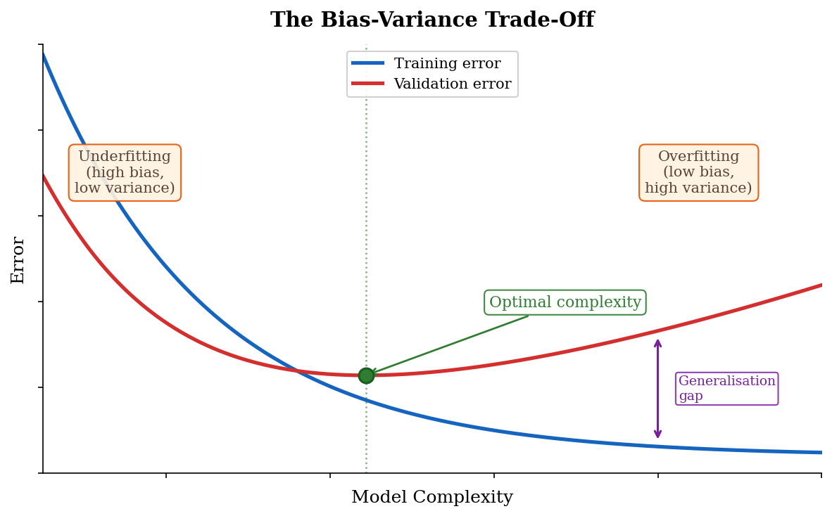
As model complexity increases — measured by the number of parameters, the degree of a polynomial, or the depth of a tree — the training error decreases monotonically. A more complex model can always fit the training data at least as well as a simpler one, and often much better. The validation error, however, follows a U-shaped curve: it decreases initially as the model gains enough complexity to capture the true pattern, reaches a minimum at the optimal complexity, and then increases as the model begins to fit noise in the training data. The gap between training error and validation error is the hallmark of overfitting: the model performs well on data it has seen and poorly on data it has not.
Regularisation techniques narrow this gap by penalising model complexity during training. L2 regularisation (also called weight decay) adds a term λ ‖w‖² to the loss function, which penalises large parameter values and encourages the model to use small weights. From a Bayesian perspective, L2 regularisation is equivalent to placing a Gaussian prior on the parameters — expressing a belief that parameter values close to zero are more probable. L1 regularisation adds λ ‖w‖₁ (the sum of the absolute values of the weights), which not only penalises large values but actively drives some weights to exactly zero, producing a sparse model that effectively performs automatic feature selection. The hyperparameter λ controls the strength of regularisation: too small, and it has no effect; too large, and it constrains the model so aggressively that it underfits.
Early stopping is another form of regularisation that exploits the dynamics of training. During gradient descent, the model's predictions typically improve on both training and validation data in the early epochs, as the model learns the dominant patterns. In later epochs, training error continues to decrease but validation error begins to rise, as the model starts to memorise noise. Early stopping halts training at the epoch where validation error is lowest, preventing the model from entering the overfitting regime. It is simple, effective, and widely used.
Trees, Ensembles, and the Non-Neural Tradition
Decision Trees: Learning by Splitting
Not all machine learning models are based on continuous optimisation of differentiable functions. Decision trees take a fundamentally different approach: they partition the feature space by asking a sequence of yes-or-no questions about individual features, and they assign a prediction to each region of the partition.
A decision tree for classifying whether a loan applicant will default might first ask: is the applicant's income above a certain threshold? If yes, it might then ask: is their credit score above 700? If no (income below the threshold), it might instead ask: do they have more than two existing loans? Each question splits the data into two groups, and the process continues recursively until some stopping criterion is met — a maximum depth, a minimum number of examples in a leaf, or a threshold below which further splitting does not improve the fit.
The result is a tree-shaped structure where each internal node represents a feature and a threshold, each branch represents the outcome of the comparison, and each leaf represents a prediction. For classification, the prediction at a leaf is typically the majority class among the training examples that reached that leaf. For regression, it is the mean of the target values.
The algorithm for building a decision tree is greedy: at each node, it considers all possible features and all possible thresholds, and selects the split that most reduces the impurity of the resulting child nodes. Impurity is measured by criteria such as the Gini index (which quantifies how often a randomly chosen example from a node would be misclassified if labelled according to the distribution of classes at that node) or entropy (which quantifies the information content of the class distribution). The optimal split at each node is chosen independently, without any gradient computation or iterative optimisation — the tree is built top-down in a single pass through the data.
Decision trees have several attractive properties. They handle both numerical and categorical features naturally, requiring no feature scaling or normalisation. They are inherently interpretable: the prediction for any input can be traced through a sequence of human-readable questions, which makes them valuable in domains where explainability is legally or ethically required, such as medical diagnosis and credit scoring. They can capture nonlinear relationships and feature interactions without explicit feature engineering, because the recursive splitting process implicitly creates regions of the feature space that correspond to conjunctions of conditions on different features.
Their weakness is instability. Because the greedy splitting algorithm makes each decision based on the data available at that node, small changes in the training data — removing a few examples, adding noise to a feature — can lead the algorithm to choose a different split at the root, which cascades into a completely different tree structure below. Deep trees, with many levels of splitting, tend to overfit severely: each leaf contains only a handful of training examples, and the tree has effectively memorised the training data rather than learning generalisable patterns. Pruning — removing branches that do not improve validation performance — mitigates this, but the fundamental instability of individual trees remains.
Random Forests and Bagging
The instability of individual decision trees is precisely what makes them amenable to a powerful variance-reduction technique called bagging (bootstrap aggregating), introduced by Breiman in 1996. The idea is to train many trees, each on a different random subset of the training data, and combine their predictions by majority vote (for classification) or averaging (for regression).
Each subset is created by sampling n examples from the training set with replacement — a procedure called bootstrapping. Because sampling is done with replacement, each subset contains roughly 63 percent of the unique training examples (some appear multiple times, others not at all), and each tree sees a slightly different version of the data. The trees are trained independently, with no communication between them, and their predictions are aggregated only at the end.
A random forest extends bagging with one additional source of randomness: at each split in each tree, only a random subset of the available features is considered as candidates for the split. This forces the trees to use different features and learn different aspects of the data, further reducing the correlation between trees and improving the ensemble's generalisation. The number of candidate features at each split is a hyperparameter, typically set to √(d) for classification and d/3 for regression, where d is the total number of features.
The effect of aggregating many diverse trees is dramatic. Individual trees are high-variance estimators: each one overfits in its own idiosyncratic way. But the errors of different trees tend to be uncorrelated (because they are trained on different data subsets and consider different features), and averaging uncorrelated errors reduces variance without increasing bias. A random forest of several hundred trees typically achieves substantially better generalisation than any single tree, at the cost of losing the interpretability of individual trees — the ensemble as a whole cannot be traced to a single chain of reasoning.
Gradient Boosting: Learning from Mistakes
Where bagging reduces variance by averaging independent models, boosting reduces bias by training a sequence of models, each focused on correcting the errors of its predecessors. Gradient boosting, formalised by Friedman in 2001, is the most successful variant and has been the dominant algorithm in machine learning competitions on structured data for over a decade.
The algorithm begins by fitting a simple model — often a single decision tree with very few splits, called a stump — to the training data. This model will have high bias and make systematic errors. The key insight of gradient boosting is to train the next tree not on the original labels, but on the residuals — the differences between the true labels and the current ensemble's predictions. The residuals quantify exactly where the current ensemble is wrong, and a tree trained to predict the residuals learns a correction that, when added to the ensemble's output, reduces the error.
Formally, at each step m, gradient boosting fits a new tree hₘ(x) to the negative gradient of the loss function evaluated at the current ensemble's predictions. For squared-error loss, the negative gradient is simply the residual y - Fₘ₋₁(x), where Fₘ₋₁ is the prediction of the ensemble after m-1 trees. For other loss functions, the negative gradient plays the same role that residuals play for squared error — it indicates the direction in which the prediction should change to reduce the loss.
The ensemble's prediction after M trees is the sum:
where ηₘ is a learning rate (often called the shrinkage parameter) that controls how much each tree's contribution is scaled down. Using a small learning rate with many trees tends to produce better generalisation than using a large rate with few trees, because it allows the ensemble to make many small corrections rather than a few large ones.
Modern implementations of gradient boosting — XGBoost (Chen and Guestrin, 2016), LightGBM (Ke et al., 2017), and CatBoost (Prokhorenkova et al., 2018) — incorporate sophisticated engineering for speed, memory efficiency, and regularisation, and they remain the algorithms of first resort for tabular prediction tasks in industry and competition settings. On datasets where the features are pre-defined numerical or categorical attributes (as opposed to raw images, audio, or text), gradient-boosted trees frequently match or exceed the performance of neural networks, with faster training and less sensitivity to hyperparameter choices.
Preparing for Depth
From Feature Engineering to Feature Learning
Throughout this material, the features presented to the model have been assumed to be given: pixel values, word frequencies, numerical measurements, one-hot encodings of categories. The process of designing and selecting these features — feature engineering — has historically been the most time-consuming and expertise-dependent part of building a machine learning system. A computer vision engineer might spend months designing edge detectors, texture descriptors, and colour histograms before training a classifier on top of them. A natural-language processing researcher might invest similar effort in defining syntactic features, part-of-speech tags, and handcrafted sentiment indicators. The quality of the features determined the ceiling on the model's performance: no amount of training could compensate for features that failed to capture the relevant structure in the data.
The limitation of handcrafted features is that they encode human assumptions about what matters. An edge detector designed to find horizontal and vertical edges will miss diagonal edges, curved contours, and texture boundaries unless additional detectors are added for each case. A bag-of-words text representation captures which words appear but not how they relate to each other, missing the distinction between "not bad" (positive sentiment) and "bad" (negative sentiment). Every domain has examples of patterns that are obvious to human perception but difficult to encode as explicit feature computations.
The promise of representation learning — the idea that the model should learn its own features from data, rather than having them prescribed by a human — was articulated early in the history of machine learning but not realised at scale until deep networks became trainable. A deep neural network with multiple hidden layers can be understood as performing automatic feature engineering: each layer transforms its input into a representation that is incrementally more useful for the task at hand. The first hidden layer might learn to detect simple patterns analogous to the features a human engineer would design. Subsequent layers combine these simple patterns into more complex and abstract representations that no human would think to construct. The learned features are not interpretable in the same way that handcrafted features are — they are high-dimensional vectors of activations with no obvious semantic meaning — but they capture structure in the data more effectively than anything a human typically designs.
The Computational Demand of High-Dimensional Problems
The models discussed in this material — linear regression, logistic regression, decision trees, random forests, gradient boosting — all work well when the number of informative features is moderate and the features themselves are meaningful. When the raw input is a high-dimensional object such as an image, a waveform, or a document, these models face a challenge that is partly statistical and partly computational.
The statistical challenge is the curse of dimensionality. In high-dimensional feature spaces, data points become sparse: the volume of the space grows exponentially with the number of dimensions, and the number of training examples needed to cover the space adequately grows with it. A model that works well in 10 dimensions may fail in 10,000 dimensions because the training data, however large, occupies only a negligible fraction of the possible feature combinations. Distances between points lose their discriminative power — in very high dimensions, the nearest neighbour and the farthest neighbour of any given point tend to be nearly the same distance away — and the simple geometric intuitions that guide model design in low dimensions break down.
The computational challenge is that processing raw high-dimensional inputs is expensive. A colour image of 224 × 224 pixels has 224 × 224 × 3 = 150,528 features. Training a logistic regression model on this input requires learning 150,528 weights plus a bias — feasible, but the model is still linear and therefore incapable of capturing the spatial structure of the image. Polynomial feature expansion to even degree 2 would produce over 11 billion features, which is intractable. Decision trees and ensembles can in principle handle high-dimensional inputs, but they typically split on one feature at a time and require an enormous number of splits to capture the spatial correlations that make images interpretable.
What is needed is a model that can handle high-dimensional inputs efficiently by exploiting the structure of the data — spatial correlations in images, sequential dependencies in text, hierarchical composition in both — rather than treating each input dimension as an independent feature. This is exactly what deeper architectures provide. Convolutional layers exploit spatial locality. Recurrent layers exploit sequential order. And the depth of the network exploits the compositional structure of natural data, building complex features from simple ones in a hierarchy of learned transformations.
Why Depth Became the Answer
The trajectory of this material has traced a path from specific failures of linearity, through the probabilistic and optimisation foundations that make learning possible, through the classical non-neural algorithms that dominated practice for decades, and finally to the question of what lies beyond. The common thread is a tension between the expressiveness of the model and the feasibility of learning.
Linear models are maximally feasible — convex loss, guaranteed convergence, interpretable weights — but insufficiently expressive. Polynomial feature expansion increases expressiveness but at a combinatorial cost in parameters and a catastrophic cost in generalisation. Decision trees are expressive and interpretable but unstable. Ensembles of trees are expressive and stable but operate on predefined features and struggle with raw high-dimensional inputs. Each approach hits a wall, and the wall is always the same: the model's features are fixed by the designer, and the model's capacity to discover new features from data is limited or absent.
Neural networks break through this wall by making the features themselves learnable. A multi-layer perceptron with one hidden layer and a nonlinear activation function can, in principle, approximate any continuous function — the Universal Approximation Theorem guarantees this. But it is depth that makes the approximation practical: a deep network with many layers can represent the same function with exponentially fewer parameters than a shallow one, because it can decompose the function into a hierarchy of simpler computations, each layer building on the representations constructed by the layer below. The features learned by the early layers are simple and local; the features learned by the later layers are complex and global; and the entire hierarchy is trained end-to-end by backpropagation, which distributes the learning signal from the output back through every layer of the representation.
The transition from handcrafted features to learned features, from shallow models to deep models, and from fixed representations to adaptive representations is the defining shift in the history of machine learning. It is a shift that did not happen overnight: the theoretical foundations were laid in the 1980s and 1990s, the key algorithmic insights accumulated through the 2000s, and the practical realisation required hardware advances — particularly the repurposing of graphics processing units for matrix computation — that only became available in the early 2010s. But once the conditions aligned, the results were dramatic. AlexNet's victory in the 2012 ImageNet competition demonstrated that a deep convolutional network trained end-to-end on raw pixels could outperform every system built on decades of handcrafted visual features by a margin that shocked the computer vision community. The lesson generalised rapidly to speech, to text, and eventually to scientific domains from protein folding to weather prediction.
Everything that follows — activation functions, backpropagation, convolutional networks, recurrent networks, attention, transformers — is built on the insight that depth, combined with gradient-based learning, allows the model to discover what matters in the data rather than being told.